Scene Recognition

An example of a typical bag of words classification pipeline. Figure by Chatfield et al.

This project report was compiled as part of the course requirements of CS 6476 Computer Vision under Prof. James Hays

Objective

Classify a given set of images into a predefined set of scenes

Abstract Algorithm

A set of training images classified by their scenes is used to train a model to find a classification model. Once the model is obtained it is tested on the test set to verify the model.

Step 1

The images are represented using pixel values and a meaningful representation of these images is required to classify these images. We implement the tiny image representation and the bags of sift representation

Tiny Image Representation

For a baseline implementation we obtain a 16x16 pixel representation of the image and normalise it. The resized image is then vectorized and used as the feature representing the image

Step 2

For a baseline implementation of the classifier, we use the K-Nearest-Neighbour Algorithm

K-Nearest-Neighbour Algorithm

Given a feature of the image and a set of features of pre-classified images, we use the label of the K-Nearest neighbours in the feature space to decide the label for the given image.

Step 3

For better implementation of the classifier, we use Support Vector Machine Method

Support Vector Machine

At a broad-level, given a binary classification of data, Support Vector Machine finds a hyper plane that partitions the data.

For Image classification, we implement a One-Vs-All method i.e. For every class we find the hyper plane that partitions the image features as class and Not class. We hence have as many hyper planes as the number of classes that we classify into. The dot product of the hyperplane with the image feature represents the distance of the data from the partition and hence gives a rough estimate on the confidence. We use this information to determine the actual class by choosing the class whose hyper plane is the farthest from the image feature representation

Step 4

Bag of words

A fixed size of vocabulary of image features(SIFT in our case) is built using the existing training images.

For simplicity, points are sampled at a fixed distance(step size) and the SIFT representation is computed for each of them. All such SIFT features across all images are then passed through a K-Means algorithm to find a fixed number(K=vocab_size) of set of features. The set of these K vectors is to be used as the vocabulary here after.

For each training image, SIFT vectors are computed at a fixed step size(Need not be the same as that used for the vocabulary).

A histogram is computed for each image and this serves as the feature representation of the image. The histogram signifies the number of features of the image that are closest to each of the vocabulary features.

The algorithm performs better with lower step sizes but due to hardware constraints a step size of 4 with SIFT and 10 with SIFT + GIST was the lowest achievable

Dataset Used

We use the 15 scene dataset introduced in Lazebnik et al. 2006, although built on top of previously published datasets

Regularization Parameter Tuning

Regularization is employed to reduce the overfitting nature of the hyperplane. Lambda parametrizes the regularization in SVMs

Lambda	Accuracy
0.0000001	0.642
0.000001	0.645
0.00001	0.638
0.0001	0.641
0.001	0.643
0.01	0.647
0.1	0.595
1	0.609
10	0.626
100	0.573
1000	0.435
10000	0.405
100000	0.405

Extra Credit

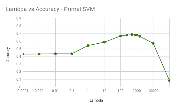
Primal SVM

As opposed to the conventional SVM, primal SVMs use the newtonian quadratic method to converge to the solution. This results in a faster convergence and more accurate hyperplane. Olivier Chapelle’s MATLAB code works well.

Lambda	Accuracy
0.0001	0.429
0.001	0.431
0.01	0.434
0.1	0.434
1	0.542
10	0.586
100	0.667
250	0.679
500	0.685
750	0.679
1000	0.679
1500	0.663
10000	0.570
100000	0.082

GIST Descriptor

Whereas SIFT provides a descriptor at a pixel level, GIST(summary) descriptor provides a high level representation of the entire image.

To use the GIST vector in our algorithm, we find the GIST representation of the image and concat it with each of the SIFT descriptors. This feature representationis used to build the vocabulary and for classifying the test image set.

Results The performance of the pipeline improved from 65% to 68% on switching to SIFT + GIST

Vocabulary Size Variation

Although it is expected that the accuracy is proportional to the vocabulary size upto a limit after which it converges, I received an unexpected result. The vocabulary size did not affect the accuracy at all. I have uploaded the vocabulary vectors in the upload package.

Results

Accuracy

Pipeline	Accuracy
Tiny Image and K-Nearest-Neighbour	0.19
Bags of Sift and K-Nearest-Neighbour	0.51
Bags of SIFT and SVM	0.68
Bags of SIFT+GIST and PRIMAL SVM	0.70

Parameters

Lambda Value for SIFT and SVM: 0.01 Lambda Value for SIFT+GIST and Primal SVM: 500

Scene Classification Results Visualization

Accuracy (mean of diagonal of confusion matrix) is 0.700

Category name	Accuracy	False positives with true label		False negatives with wrong predicted label
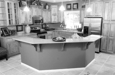
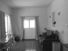
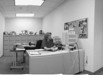
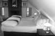
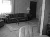
Kitchen	0.520	Industrial	Bedroom	Industrial	LivingRoom
Store	0.730	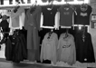OpenCountry	InsideCity	InsideCity	Office
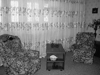
Bedroom	0.560	LivingRoom	LivingRoom	Office	LivingRoom
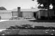
LivingRoom	0.630	InsideCity	Suburb	Bedroom	Kitchen
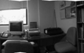
Office	0.770	Industrial	Kitchen	LivingRoom	LivingRoom
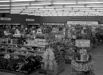
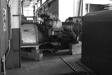
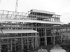
Industrial	0.490	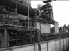InsideCity	Street	Kitchen	Store
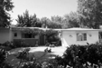
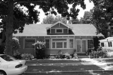
Suburb	0.930	Coast	OpenCountry	LivingRoom	Store
InsideCity	0.610	TallBuilding	Industrial	Store	Kitchen
TallBuilding	0.680	LivingRoom	Mountain	InsideCity	Industrial
Street	0.750	OpenCountry	TallBuilding	Industrial	Store
Highway	0.810	OpenCountry	Mountain	InsideCity	Coast
OpenCountry	0.580	Forest	Mountain	Highway	Forest
Coast	0.770	Highway	Mountain	Highway	OpenCountry
Mountain	0.830	OpenCountry	Coast	Coast	Highway
Forest	0.840	Mountain	Store	Street	Mountain

References

1 Oliva, A. & Torralba, A. International Journal of Computer Vision (2001) 42: 145. 2 L. Fei-Fei and P. Perona, “A Bayesian hierarchical model for learning natural scene categories,” 2005 IEEE Computer Society Conference on Computer Vision and Pattern Recognition (CVPR’05), 2005, pp. 524-531 vol. 2.