Hidden Markov Model is a sequence model: A model which assigns a label or class to each unit in a sequence, thus mapping a sequence of observations to a sequence of labels.

• Hidden: The states that the observations are emitted from are unknown(hidden)
• Markov: The model follows the Markovian assumption that any state is dependent only on its prior state

For example: Given the humidity values of a sequence of days, we can guess whether it rained on those days.

The Model

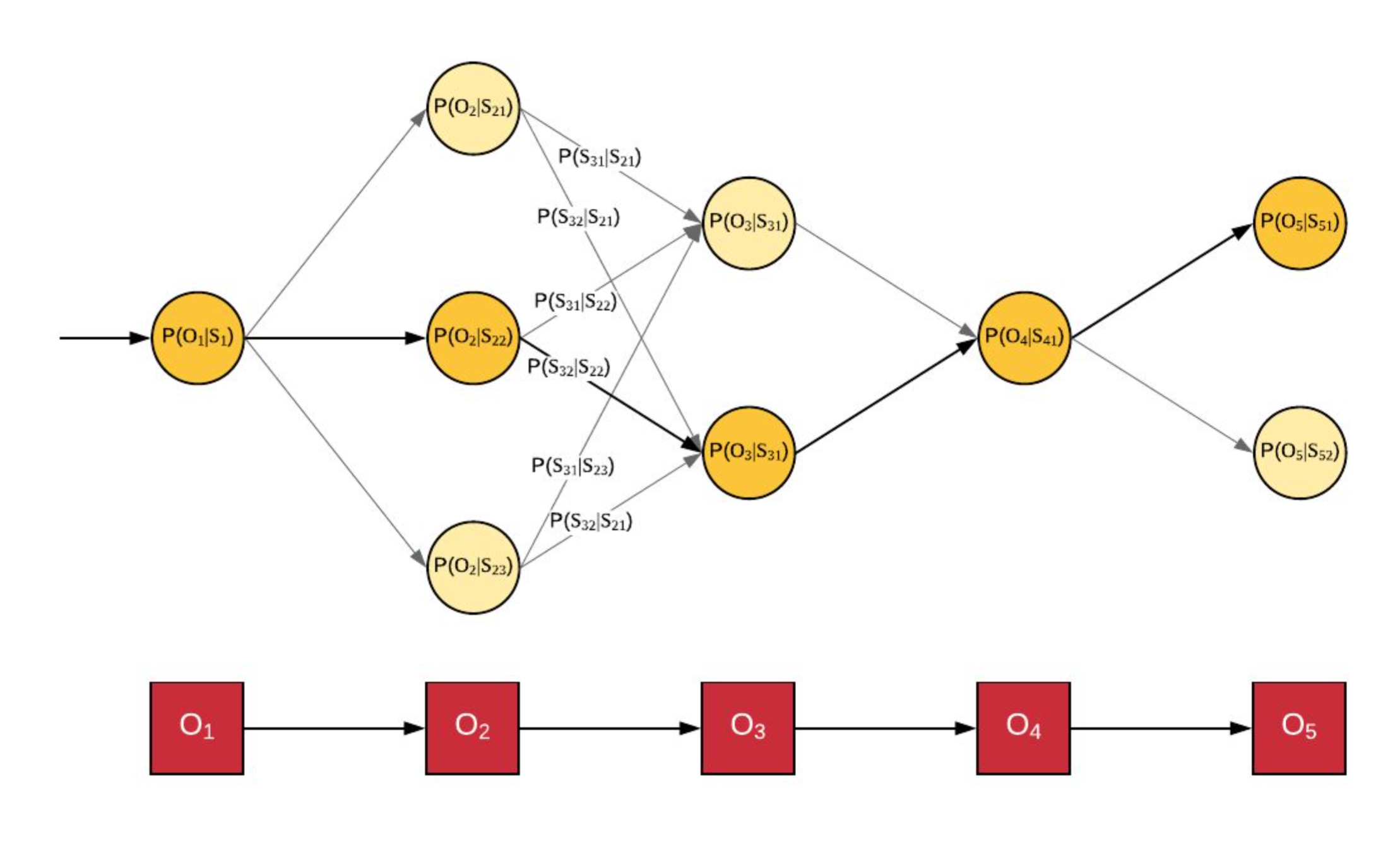
A hidden markov model comprises of

• Observations: Sequence of observed values \((O_i): [O_1, O_2, \ldots , O_n]\)
• States: Each observation \(O_i\) has \(m_i\) potential matching states.
  \((S_{i,j}): [S_{1,1}, S_{1,2}, \ldots , S_{1,m_1}, S_{2,1}, S_{2,2}, \ldots , S_{2,m_2}, \ldots, S_{n,1}, S_{n,2}, , S_{n,m_n}]\)
• Model Parameters
  • Emission Probability: Probability of observing \(O_i\) in state \(S_{i,j}\) i.e. \(P(O_i \vert S_{i,j})\)
  • Transition Probability: Probability of occurence of state \(S_{i+1,j}\) after \(S_{i,j}\). i.e. \(P( S_{i+1,j} \vert S_{i,j} )\)

An illustration of the Hidden Markov Model. Each circle S_i​,j ​represents a state, while O_i​s represent the observations. The highlighted path is the path of maximal likelihood as determined by Viterbi Algorithm.

In an influential survey, Rabiner (1989) defines three problems for Hidden Markov models:

1. Likelihood: Computing the marginal probability of the occurence of a sequence of observations
   Algorithms: Forward Algorithm, Backward Algorithm
2. Decoding: Computing the most likely sequence of states that generated the observations
   Algorithms: Viterbi Algorithm
3. Training: Estimating the model parameters (emission and transition probabilities) given the model and the sequence of observations
   Algorithms: Baum Welch (Forward-Backward Algorithm), Maximum Likelihood Estimation

Viterbi Algorithm

The Viterbi algorithm is a dynamic programming algorithm for finding the most likely sequence of hidden states — called the Viterbi path — that results in a sequence of observed events.

$$ V_{t,k} = P(O_t | S_{t,k}) \times \max_{x \in S} \{ P(S_{t, k} | S_{t-1, x} ) \times V_{t-1,x} \} $$

where \(V_{t,k}\): is the total probability of observing \(O_t\) from state \(S_{t,k}\)

Applications

HMMs are an excellent tool to guess the sequence of events that led to a given sequence of noisy signals. HMMs find their applications in multiple domains

Map Matching

I spent my Summer, interning in the Maps Division at Uber. I was intrigued to find out that HMMs are used in the industry and in a very crucial piece of the Uber’s product line - Map Matching. Map matching is the problem of matching GPS Locations to a logical map model.

The driver’s app periodically emits its GPS signal to the Uber servers. This GPS signal is used by Uber to locate and match with the drivers actual location on the Map.
Sounds too simple right? Guess what? Its not!

How GPS works
GPS is a network of about 30 satellites orbiting the Earth in a such a way that at any point on the earth at least 4 satellites are in direct line of sight. Periodically, the satellites emit their positions and current time. These signals are intercepted by a GPS receiver to compute the exact GPS location based on the speed of the signal and the time delay between the signals.

GPS is inherently a noisy signal. The noise can be due to the atomic clocks, the computation time and the receiver precision; but none of these cause as much error as tall buildings. Areas of tall buildings (also called urban canyons) cause the signal to be reflected on the buildings and hence cause large deviations in the computed GPS locations.

HMMs to the rescue

It is due to these errors that HMMs find use in map matching.

Based on the works of Paul Newson and John Krumm:

• States: Each state is the snapped GPS location on the logical map model. Based on the approximate error in GPS locations, a set of potential GPS locations is generated by scanning for all points in a fixed neighbourhood.
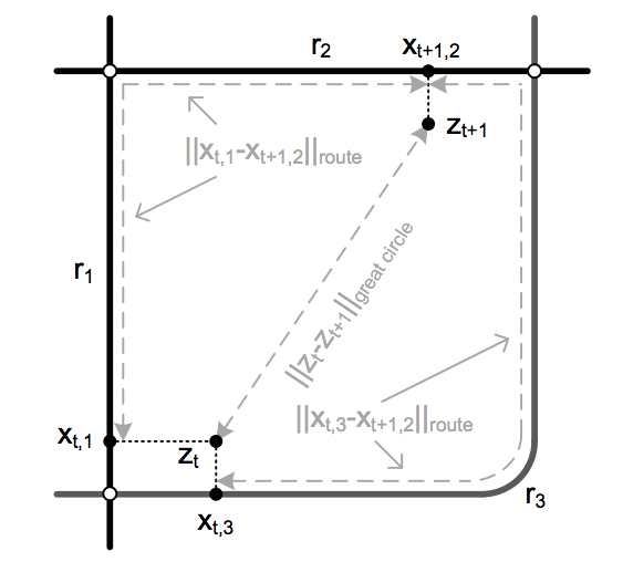
• Emission Probability: The emission probability is inversely proportional to the distance between the observed GPS location and the GPS location of the potential candidate on the map model.

$$ p(z_t \vert r_t) = \frac{1}{\sqrt{2 \pi} \sigma_z} e^{ -0.5\Big (\frac{\Vert z_t - x_{t, i} \Vert_{great\ circle}}{\sigma_z}\Big )^2} $$

where \(z_t\): Map location of observed GPS signal
\(r_t = \Vert x_{t, 1} - x_{t+1, 2} \Vert _{route}\): Road segment length
\(x_{t, i}\): Map location of potential candidate
\(\sigma_z\): Estimated hyperparameter

• Transition Probability: Transition probability is inversely proportional to the distance between the transitioning states and the routing distance between the observations

$$ p(d_t) = \frac{1}{\beta} e^{-d_t} \\ d_t= \Vert s_t -s_{t + 1}\Vert_{great\ circle} - \Vert x_{t, i*} -x_{t + 1, j*} \Vert_{route} $$

This shows an example of the notation. There are three road segments, r₁, r₂, and r₃, and two measured points, z_t and z_t+1. The first measured point, z_t, has candidate road matches at x_{t, 1} and x_{t, 3} . Each match candidate results in a route to x_{t+1, 2}, which is a match candidate for the second measured point, zt+1. These two routes have their own lengths, as does the great circle path between the two measured points. Our data shows that the route distance and great circle distance are closer together for correct matches than for incorrect matches. Source

---

Sequence Labeling in Natural Language

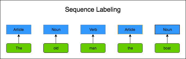
A popular Natural Language problem is Part of Speech(POS) Tagging - assigning POS to each word in a sentence.

Emission and transition probabilities are estimated using heuristics like

• Maximal likelihood estimation
• Baum Welch (Forward-Backward Algorithm)

More details in this post

---

Morse Code Decoding

Given a stream of noisy audio samples we can identify the embedded morse code using HMMs. Assume, for instance that you have the noise priors.

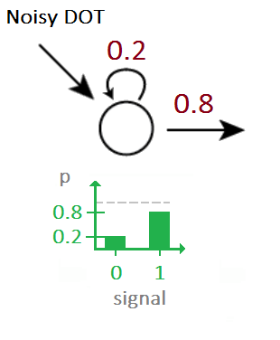
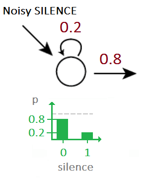
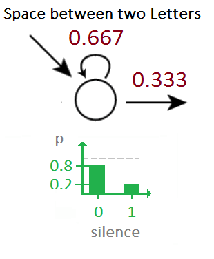
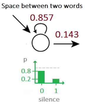
Given a stream of noisy morse code signals, we can now use HMMs to to find the underlying sequence of Morse codes by using the above as the emission probabilities.